SMALL EXPERIMENT · SIGNALS & INTERCONNECTS
Watching a signal travel down a cable
A wire is easy to treat as an instant connection until the scope shows otherwise. Nishant and I sent square waves down a 15-meter coaxial cable and watched both ends. Changing what was connected to the cable made the same edge arrive, reflect, and settle in very different ways.
The delay is real
We started with a square wave around 200 kHz. The important timescale here is the edge speed, not just the time between pulses: if an edge changes substantially while it is still traveling, the cable needs to be treated as a transmission line.
The generator measured 2.01 V unloaded and 1.00 V with a 50 Ω load. Treating its output as a voltage source with a series resistance gives 50 × (2.01 / 1.00 − 1) = 50.5 Ω, close to the cable’s roughly 50 Ω characteristic impedance. Characteristic impedance describes the voltage-to-current ratio of a traveling wave; it is not the cable’s DC resistance.
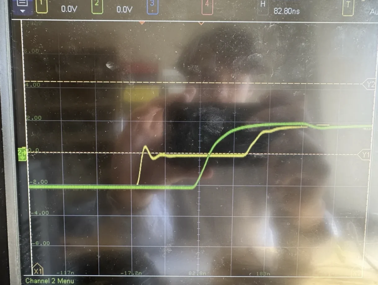
With the far end open, the near-end trace showed an initial step and then the returning reflection about 145 ns later. That is a round trip. Dividing twice the 15 m length by that delay gives a propagation speed of about 2.07 × 10⁸ m/s, or 69% of the speed of light.
Giving the wave somewhere to go
At an open end, current cannot keep flowing into a load. The reflected voltage has the same polarity as the arriving wave, so the two add at the endpoint. Back at the source, the returning wave changes the voltage only after the cable’s round-trip delay.
Putting 50 Ω at the far end made the traces much cleaner. A matching load absorbs the incoming wave, leaving very little reflection. The far-end trace becomes approximately a delayed version of the near-end trace. The reflection coefficient, Γ = (Rload − Z0) / (Rload + Z0), describes this: an open circuit approaches +1, a short gives −1, and a matched load gives zero.
Changing the source and the load
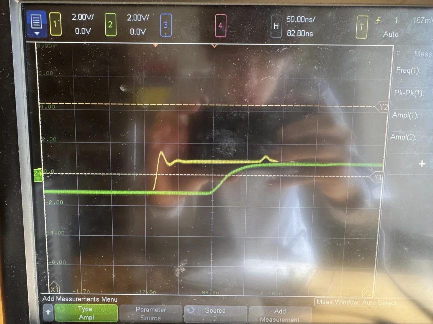
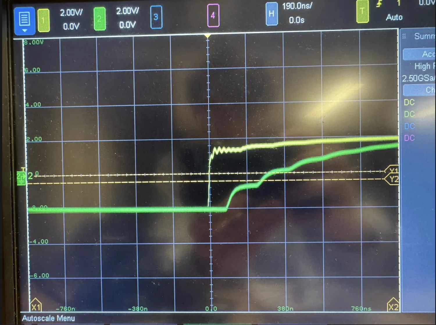
We reopened the far end and added 220 Ω in series at the source. That reduced the initial launched wave and made the source a poor match for a returning reflection. The expected source reflection coefficient is about +0.69, so repeated bounces produce a staircase toward the final voltage. With 20 Ω added instead, the expected coefficient is about +0.17, and the secondary steps are much less pronounced.
A 1 nF capacitor at the far end behaves differently again. Its voltage cannot change instantly, so the first part of an edge sees a load resembling a short. As it charges, current falls and the load tends toward an open circuit. That changing response rounds the far-end edge and sends a time-varying reflection back toward the source.
Logic outputs are analog circuits too
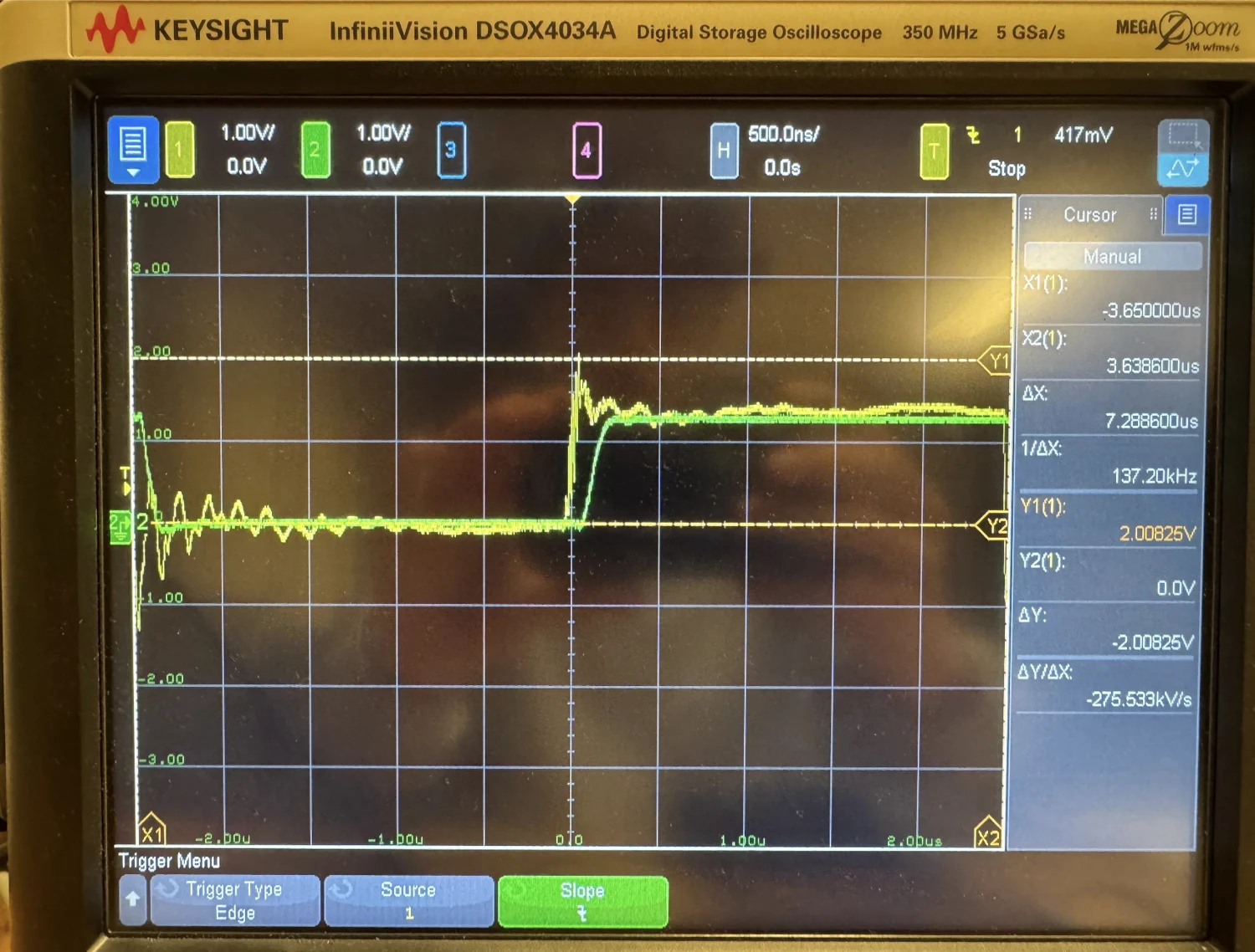
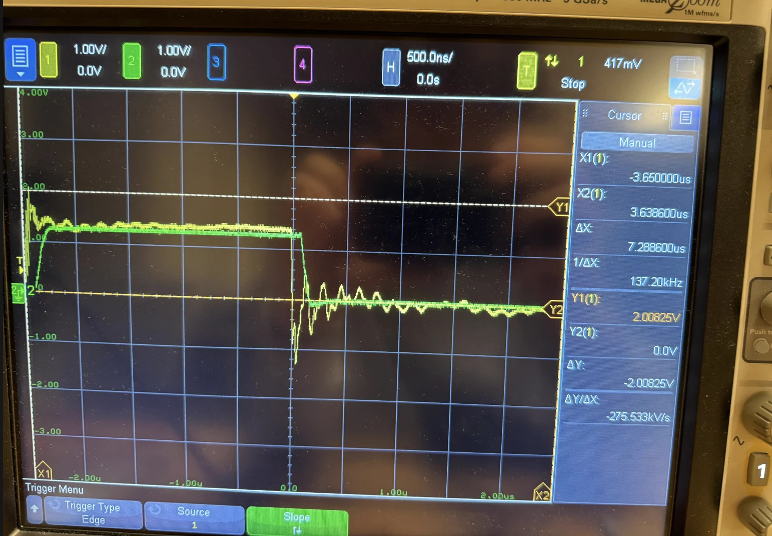
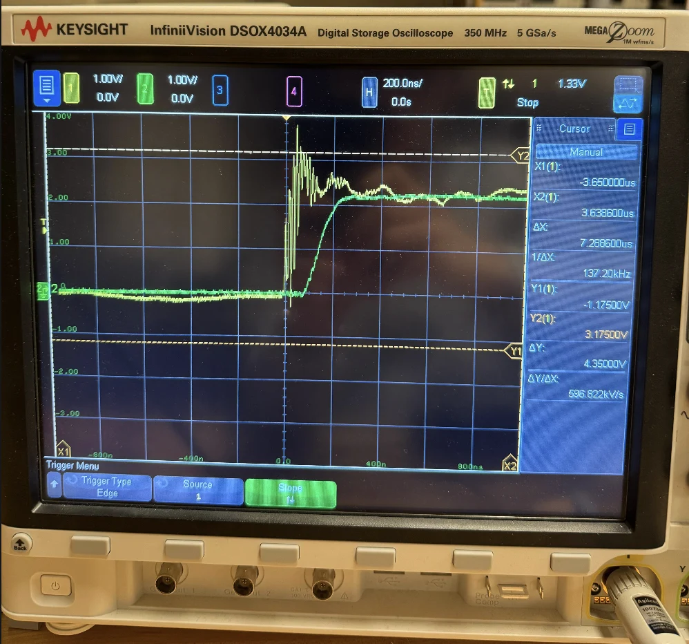
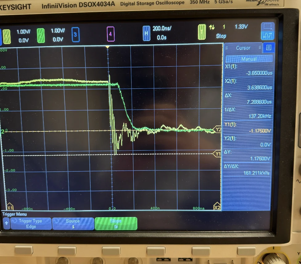
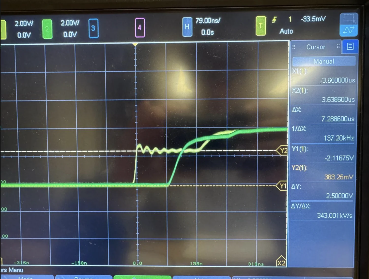
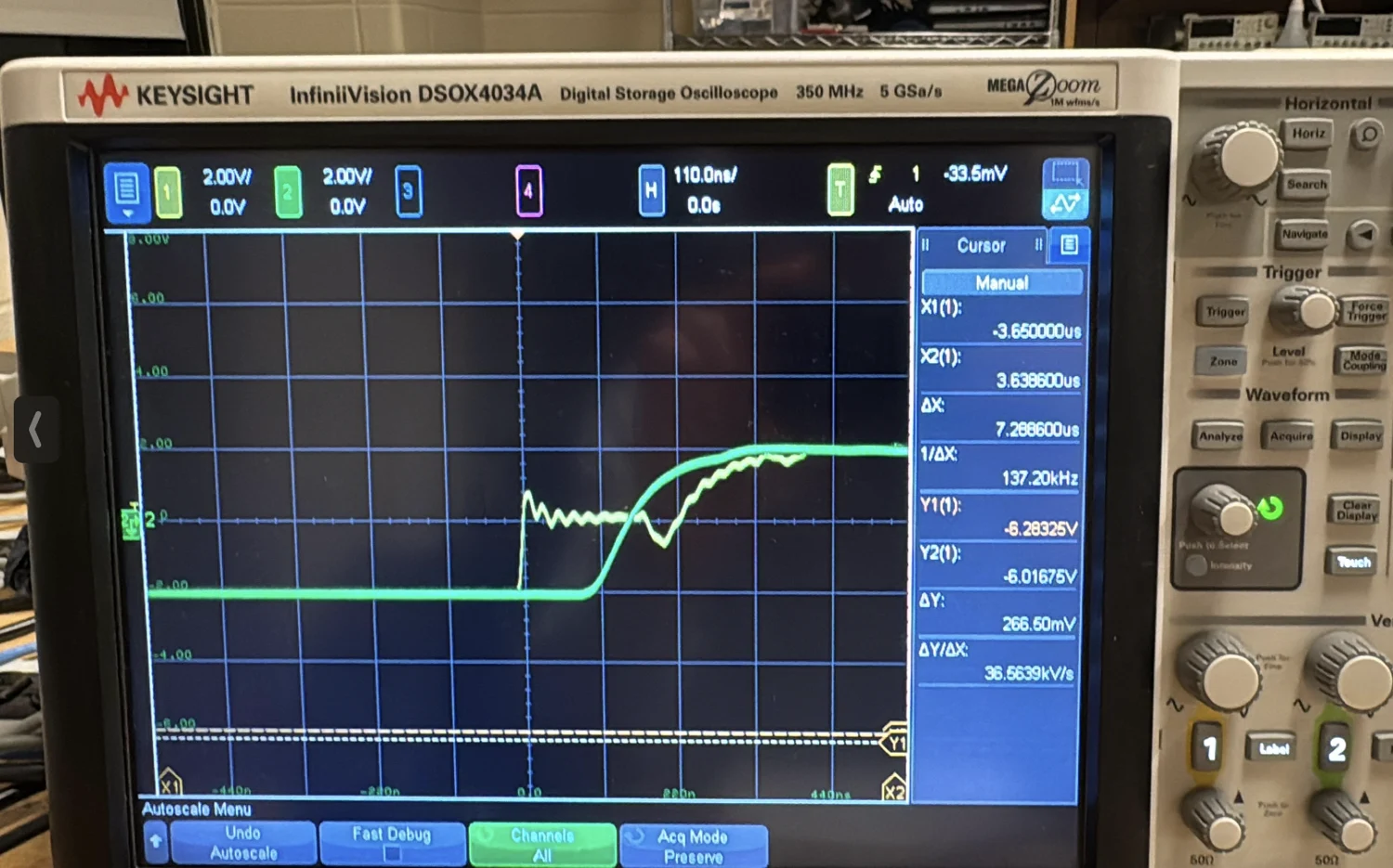
Finally, we drove the cable with TTL and CMOS inverters. The 74F04 TTL driver showed noticeably different rising and falling behavior: pulling a line low and driving it high do not use equally strong output paths. The 74HC04 CMOS driver was more balanced, although its traces still showed transients.
These captures are a useful comparison, rather than precise measurements of fixed output resistances. A logic driver is nonlinear, and estimating its impedance from a transient depends on which voltage and point in time are being measured. For me, the useful connection is that a digital “one” still has to travel through a real analog circuit before another device can read it.