SMALL EXPERIMENT · CONVERSION & SAMPLING
An analog signal’s round trip
Signal processing depends on being able to turn a changing voltage into numbers. I wanted to see that boundary directly, so Nishant and I built a digital voltage display and connected an analog-to-digital converter to a digital-to-analog converter. Watching both sides on the scope made the limits much easier to see.
A clock is not a sample rate
An ADC assigns a binary code to an input voltage. Its reference range sets which voltages fit, and its bit depth sets how many distinct levels it can represent. An 8-bit converter has 256 possible codes, so even a steady voltage gets rounded into a finite-sized step.
Our measured converter clock was 230.91 kHz, with a period of about 4.33 µs. A conversion took about 298.35 µs, or roughly 69 clock cycles. The converter needs multiple clock cycles to produce each result, so it was not taking 230,910 samples per second. Using the measured conversion interval gives about 3,352 conversions per second. We did not observe that interval changing with the input voltage.
Displaying a voltage in octal
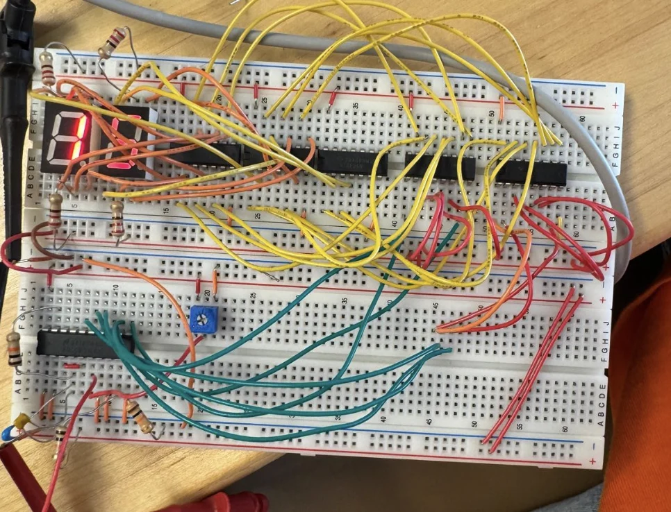
We used six bits for a two-digit octal readout. Octal is base eight: each digit corresponds to three binary bits, so two groups of three can represent 00 through 77, or 0 through 63 in decimal. Keeping the upper six bits of an 8-bit result trades resolution for a simpler display.
The signal path was ADC, segment drivers, inverters, then the displays. The drivers turn a three-bit value into the pattern of illuminated segments; the inverters adapt the segment logic to the display connections. Across a nominal 0–5 V span, 64 levels put the display step size around 78 mV. This is a voltage represented as a code, rather than a direct decimal reading in volts.
The breadboard display worked, but my saved test table contains transcription inconsistencies, including an “8” in an octal value. I would need to repeat those readings before using them to claim an accuracy figure.
Back to a waveform
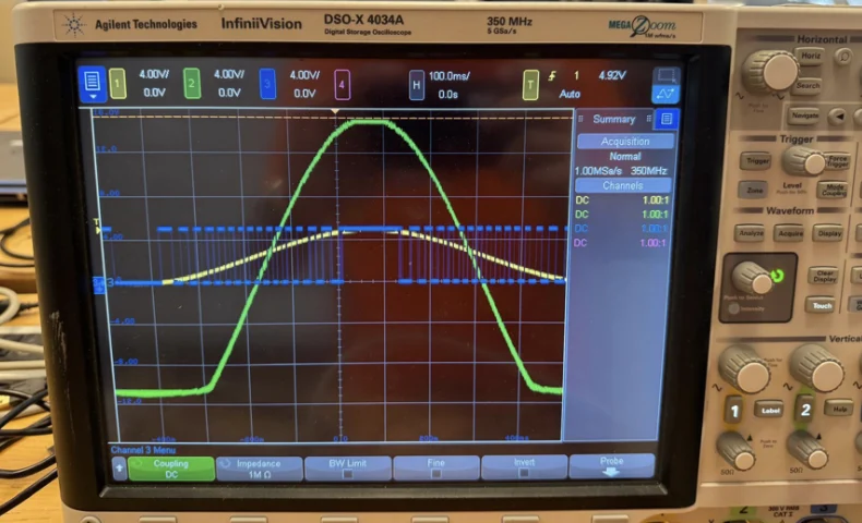
Next, the ADC’s digital output drove a DAC. The DAC turns each code back into an analog level, holding a value until the next update. At 100 Hz there are about 33 samples per cycle, enough to follow the sine wave’s shape. The output still has discrete steps; a reconstruction filter would smooth those steps and reduce the extra high-frequency content.
Increasing the amplitude eventually clipped the reconstructed waveform. A signal outside the conversion chain’s usable range cannot be represented correctly, regardless of how slowly it changes. Clipping is an amplitude limit, separate from the timing limit that causes aliasing.

When faster looks slower
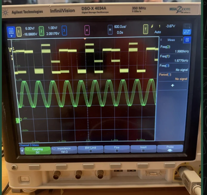
At our estimated sample rate, the Nyquist boundary is about 1.676 kHz. As the input approaches it, there are only about two samples per cycle. That leaves little information about the waveform between samples, and operation exactly at the boundary is sensitive to phase.
Above that boundary, different input frequencies can produce the same sequence of samples. For an ideal 3.352 kHz sampling rate, a 1.8 kHz sine folds to about 1.552 kHz, and a 2 kHz sine to about 1.352 kHz. These are calculated aliases, not frequencies established by the scope photographs. The automatic frequency readings on the distorted output should not be taken as a reliable measurement of its fundamental.
This is why an anti-aliasing filter goes before the ADC: it removes unwanted frequencies before sampling makes them indistinguishable from lower ones. Once the information has folded together, filtering the output cannot tell which input produced it.